Tjur's R2 in JAGS

A coefficient of discrimination to assess model performance

Florencia Grattarola

Last updated on 8 February 2023 4 min read

I recently jumped into Bayesian analysis and Integrated Species Distribution Modelling. Here’s the preprint out of an amazing collaboration with Diana Bowler and Petr Keil: ‘Integrating presence-only and presence-absence data to model changes in species geographic ranges: An example of yaguarundí in Latin America’. 🐈 🌎 ⏳

The are no standard methods to assess the performance of these models, yet posterior predictive checks are a good option. For our model we needed a statistic that fitted a binomial regression, to assess the performance on the presence-absence data. A nice and simple metric for this is Tjur’s coefficient of discrimination $D$ (Tjur 2009).

This pseudo R square value compares the average fitted probability $\psi$ of the two response outcomes (1=presence or 0=absence):

$R^2Tjur = \dfrac{1}{n_1} \sum(\psi[Y=1]) - \dfrac{1}{n_0} \sum(\psi[Y=0])$

If the model has perfect discriminating power, then $R^2Tjur$ will equal 1. If the model has no discriminating power, then $R^2Tjur = 0$.

Code

Here I provide the code to assess the performance of a model with a binomial response that is included directly in the JAGS code. This was inspired by the work of Viana, Keil, & Jeliazkov and their R2D2 functions. The code to simulate the data was adapted from code written by Petr Keil.

library(spatstat)
library(sp)
library(maptools)
library(rgeos)
library(raster)
library(gstat)
#-------
library(jagsUI) # interface to JAGS
library(tidyverse)

Data simulation

# make randomness reproducible
set.seed(1234567)  

#--------------------------------------------------------------------
# Environment
size=100
env <- im(matrix(0, size, size), xrange=c(0,1), yrange=c(0,1))
xy <- expand.grid(x = env$xcol, y = env$yrow)
g.dummy <- gstat(formula=z~1, locations=~x+y, dummy=T, beta=0,
                 model=vgm(psill=0.1, range=50, model='Exp'), nmax=20)
env <- predict(g.dummy, newdata=xy, nsim=1)

sp::gridded(env) <- ~x+y
env <- as.im(raster(env))
# scale the env. variable
env <- (env - min(env))
env <- env / max(env)

#--------------------------------------------------------------------
# Parameters
alpha <- 0  # intercept of the environment-intensity relationship
beta <- 10 # slope of the environment-intensity relationship
true.params <- c(alpha = alpha, beta = beta)

#--------------------------------------------------------------------
# True point pattern
# point process intensity lambda as a function of environment
lambda <- exp(alpha + beta*env)

# sample points using inhomogeneous poisson point process
PTS <- rpoispp(lambda)
PTS.sp <- as(object=PTS, "SpatialPoints")

#--------------------------------------------------------------------
# Generate presence-absence survey locations (polygons)
# number of survey locations
N.surv <- 50

# generate the polygons
X <- rThomas(kappa = 50,  scale = 0.2, mu = 5, win=owin(xrange=c(0,1), yrange=c(0,1)))
PLS <- dirichlet(X)
PLS.sub <- PLS[sample(1:length(PLS$tiles), size=N.surv)]

# convert tesselation to sp class
PLS.sp <- as(PLS.sub, "SpatialPolygons")

# calculate area, coordinates, abundance, and incidence in each polygon
PLS.area <- gArea(PLS.sp, byid=T)
PLS.coords <- data.frame(coordinates(PLS.sp))

names(PLS.coords) <- c("X","Y")
PLS.abund <- unlist(lapply(X = over(PLS.sp, PTS.sp, returnList = TRUE), FUN = length))
PLS.presabs <- 1*(PLS.abund > 0)

# extract environmental variables
PLS.env <- raster::extract(x = raster(env), y = PLS.sp, fun = mean)[,1]

jags.data <- list(n = N.surv,
                  presabs = unname(PLS.presabs),
                  area = unname(PLS.area),
                  env = PLS.env)

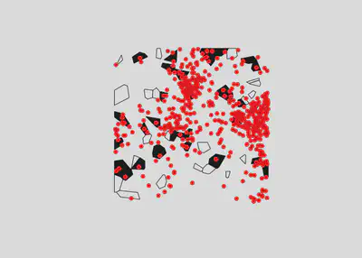
plot(PLS.sp, col = jags.data$presabs)
plot(PTS.sp, add=T, pch = 19, col = "red")

Model

cat('model
  {
    # PRIORS --------------------------------------------------

    ## Effect of sampling effort in PA data
    alpha ~ dnorm(0, 0.01)
    beta ~ dnorm(0, 0.01)

    # LIKELIHOOD --------------------------------------------------

    for (i in 1:n)
    {
        # the probability of presence
        cloglog(psi[i]) <- alpha + beta*env[i] + log(area[i])

        # presences and absences come from a Bernoulli distribution
        presabs[i] ~ dbern(psi[i])    

    # POSTERIOR PREDICTIVE CHECK  --------------------------------
    # Fit assessments: Tjur R-Squared (fit statistic for logistic regression)
        pres[i] <- ifelse(presabs[i] > 0, psi[i], 0)
        absc[i] <- ifelse(presabs[i] == 0, psi[i], 0)
    }
    # Discrepancy measures for entire data set
    pres.n <- sum(presabs[] > 0)
    absc.n <- sum(presabs[] == 0)
    r2_tjur <- abs(sum(pres[])/pres.n - sum(absc[])/absc.n)

  }
', file = 'models/r2tujr.txt')

Run

fitted.model <- jagsUI::jags(data=jags.data,
                             model.file='models/r2tujr.txt',
                             parameters.to.save=c('alpha', 'beta',
                                                  'psi', 'presabs.new',
                                                  'r2_tjur'),
                             n.chains=3,
                             n.iter=10000,
                             n.thin=1,
                             n.burnin=1000,
                             parallel=TRUE,
                             DIC = FALSE)

##
## Processing function input.......
##
## Done.
##  
## Beginning parallel processing using 3 cores. Console output will be suppressed.
##
## Parallel processing completed.
##
## Calculating statistics.......
##
## Done.

Checks

psi <- fitted.model$mean$psi
presabs <- jags.data$presabs
pred <- data.frame(presabs, psi)

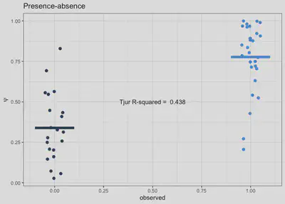
r2_tjur <- round(fitted.model$mean$r2_tjur, 3)

ggplot(pred, aes(x=presabs, y=psi, col=presabs)) +
  geom_jitter(height = 0, width = .05, size=2)  +
  scale_x_continuous(breaks=seq(0,1,0.25)) + scale_colour_binned() +
  labs(x='observed', y=latex2exp::TeX('$psi$'), title='Presence-absence') +
  stat_summary(
    fun = mean,
    geom = "errorbar",
    aes(ymax = ..y.., ymin = ..y..),
    width = 0.2, size=2) +
  theme_bw() + theme(legend.position = 'none')+
  annotate(geom="text", x=0.5, y=0.5,
           label=paste('Tjur R-squared = ', r2_tjur))

R2.Tjur <- function(Y.obs, Y.pred){
  Y.obs <- as.matrix(Y.obs)
  Y.pred <- as.matrix(Y.pred)
  r2 <- numeric(ncol(Y.obs))
  for(i in 1:ncol(Y.obs)){
    r2[i] <- unname(diff(tapply(Y.pred[,i], Y.obs[,i], mean, na.rm = TRUE)))
  }
  return(r2)
}
R2.Tjur(jags.data$presabs, fitted.model$mean$psi)

## [1] 0.4380082

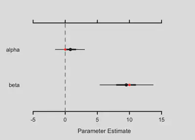
We can see if the posterior distributions of the parameters match the simulated ones

MCMCvis::MCMCplot(object = fitted.model,
  params = c('alpha', 'beta'));
  points(true.params, 2:1, pch=19, col="red")

R SDMs