two2tango

Simulation of associated virtual species

Florencia Grattarola

Last updated on 1 April 2025 4 min read

The model assumes an underlying Poisson point pattern and a Gaussian response, with intensity $λ$ of species 1 and 2 given by:

$λ_{1} = p e a k_{1} \times e x p^{(- 1 / 2 \times \frac{(t e m p - μ_{1})^{2}}{σ_{1}^{2}} + e_{1})}$
$λ_{2} = p e a k_{2} \times e x p^{(- 1 / 2 \times \frac{(t e m p - μ_{2})^{2}}{σ_{2}^{2}} + e_{2})}$

where $t e m p$ is the predictor, $μ_{1}$ and $μ_{2}$ are the niche mean for each species, and $σ_{1}$ and $σ_{2}$ represent the niche breath. The variables $p e a k_{1}$ and $p e a k_{2}$ are constants to that set the expected abundance at the mean.

Both species are associated through a residuals $e_{1}$ and $e_{2}$ :

$e_{i j} \sim MVN (0, Σ)$

Residuals have a multivariate (bivariate) normal distribution with mean zero and covariance matrix,

$Σ = [\begin{matrix} v a r_{1, 1} & c o v_{1, 2} \\ c o v_{2, 1} & v a r_{2, 2} \end{matrix}]$

The inverse of the covariance matrix is called the precision matrix, denoted by $τ = Σ^{- 1}$ .

Function

The function two2tango() needs the following arguments:

mu_1 = $μ_{1}$ and mu_2 = $μ_{2}$ : the mean of the response curve (niche mean) for each species,
sigma_1 = $σ_{1}$ and sigma_2 = $σ_{2}$ : the SD of the response curve (niche breath) for each species,
peak_1 = $p e a k_{1}$ and peak_2 = $p e a k_{2}$ : constants that set the expected abundance at the mean,
var = $v a r_{1, 1}$ = $v a r_{2, 2}$ : the variance of each species, which will always be set to 1,
cov1 = $c o v_{1, 2}$ and $c o v_{2, 1}$ : the covariance of one species against the other, which needs to be symmetric.

Then it returns a list with two sf objects of POINT geometry, one for each species.

library(spatstat)
library(tmap)
tmap_mode("plot")
library(terra)
library(gstat)
library(sf)
library(tidyverse)

# functions
source('code/two2tango.R')
source('code/auxiliary.R')

Test the function

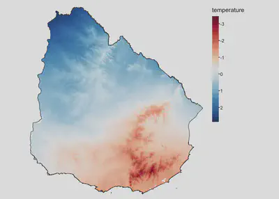
We will use as an example covariate the average annual temperature for Uruguay

uruguay <- geodata::gadm(country = 'UY', level=0, path = 'data/')
temperature <- geodata::worldclim_country('UY', var = 'tavg', path = 'data/')
temperature <- mean(temperature, na.rm=T) %>% mask(uruguay)
temp <- scale(temperature)

tm_shape(temp) +
  tm_raster(col.scale = tm_scale_continuous(midpoint = NA, values = 'brewer.rd_bu'),
            col.legend = tm_legend('temperature')) +
tm_shape(uruguay) +
  tm_borders() +
  tm_layout(frame=F, legend.frame = F)

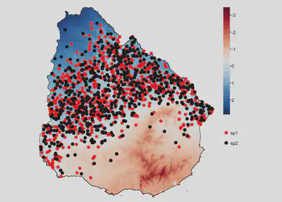
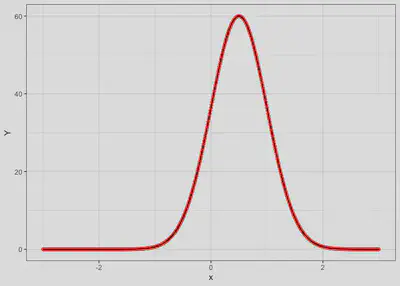
Case 1

Species have the same niche and co-occur

	$μ_{1}$	$σ_{1}$	$p e a k_{1}$	$v a r$	$c o v$
`sp1`	0.5	0.5	60	1	0.9
`sp2`	0.5	0.5	60	1	0.9

mu1 = 0.5
mu2 = 0.5
sigma1 = 0.5
sigma2 = 0.5
peak1 = 60
peak2 = 60
cov= 0.9

simulated_species <- two2tango(peak1=peak1, peak2=peak2,
                               mu1=mu1, sigma1=sigma1,
                               mu2=mu2, sigma2=sigma2,
                               cov=cov,
                               predictor = temp)

sp1 <- simulated_species[[1]] %>% mutate(species = 'sp1')
sp2 <- simulated_species[[2]] %>% mutate(species = 'sp2')

Code

tm_shape(temp) +
  tm_raster(col.scale = tm_scale_continuous(midpoint = NA, values = 'brewer.rd_bu'),
            col.legend = tm_legend('')) +
tm_shape(uruguay) + tm_borders() +
tm_shape(sp1) +
  tm_dots(fill='species',
          fill.scale = tm_scale_categorical(values='red'),
          fill.legend = tm_legend(''), size = 0.5) +
tm_shape(sp2) +
  tm_dots(fill='species',
          fill.scale = tm_scale_categorical(values='black'),
          fill.legend = tm_legend(''), size = 0.5) +
  tm_layout(frame=F, legend.frame = F)

Code

response.df <- tibble(x = seq(-3, 3, by = 0.01),
                      y1 = spec.response(x, mu1, peak1, sigma1),
                      y2 = spec.response(x, mu2, peak2, sigma2))

ggplot() +
    geom_line(data=response.df, aes(x=x, y=y1), col='red', linetype = 'dashed') +
    geom_point(data=response.df, aes(x=x, y=y1), col='red') +
    geom_line(data=response.df, aes(x=x, y=y2), col='black') +
    geom_line(data=response.df, aes(x=x, y=y2), col='black') +
    labs(y='Y') + theme_bw()

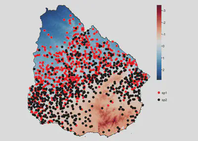
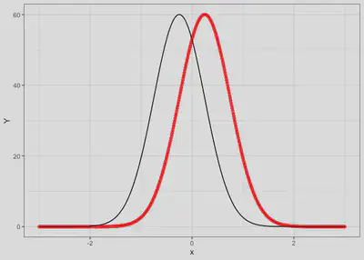
Case 2

Species have a different niche and negative co-occurrence

	$μ_{1}$	$σ_{1}$	$p e a k_{1}$	$v a r$	$c o v$
`sp1`	0.25	0.5	60	1	-0.9
`sp2`	-0.25	0.5	60	1	-0.9

mu1 = 0.25
mu2 = -0.25
sigma1 = 0.5
sigma2 = 0.5
peak1 = 60
peak2 = 60
cov= -0.9

simulated_species <- two2tango(peak1=peak1, peak2=peak2,
                               mu1=mu1, sigma1=sigma1,
                               mu2=mu2, sigma2=sigma2,
                               cov=cov,
                               predictor = temp)

sp1 <- simulated_species[[1]] %>% mutate(species = 'sp1')
sp2 <- simulated_species[[2]] %>% mutate(species = 'sp2')

Code

tm_shape(temp) +
  tm_raster(col.scale = tm_scale_continuous(midpoint = NA, values = 'brewer.rd_bu'),
            col.legend = tm_legend('')) +
tm_shape(uruguay) + tm_borders() +
tm_shape(sp1) +
  tm_dots(fill='species',
          fill.scale = tm_scale_categorical(values='red'),
          fill.legend = tm_legend(''), size = 0.5) +
tm_shape(sp2) +
  tm_dots(fill='species',
          fill.scale = tm_scale_categorical(values='black'),
          fill.legend = tm_legend(''), size = 0.5) +
  tm_layout(frame=F, legend.frame = F)

Code

response.df <- tibble(x = seq(-3, 3, by = 0.01),
                      y1 = spec.response(x, mu1, peak1, sigma1),
                      y2 = spec.response(x, mu2, peak2, sigma2))

ggplot() +
    geom_line(data=response.df, aes(x=x, y=y1), col='red', linetype = 'dashed') +
    geom_point(data=response.df, aes(x=x, y=y1), col='red') +
    geom_line(data=response.df, aes(x=x, y=y2), col='black') +
    geom_line(data=response.df, aes(x=x, y=y2), col='black') +
    labs(y='Y') + theme_bw()

R JSDM

two2tango

Function

Test the function

Case 1

Case 2

Florencia Grattarola

Postdoc Researcher